


A Pollinator in Pink……..HFDF! flickr photo by The Manic Macrographer shared under a Creative Commons (BY) license
The problem of constructing a decision tree can be expressed recursively. First, select an attribute to place at the root node and make one branch for each possible value. This splits up the example set into subsets, one for every value of the attribute. Now the process can be repeated recursively for each branch, using only those instances that actually reach the branch. If at any time all instances at a node have the same classification, stop developing that part of the tree.
The only thing left to decide is how to determine which attribute to split on, given a set of examples with different classes. If we had a measure of the purity of each node, we could choose the attribute that produces the purest daughter nodes. The measure of purity that we will use is called the information and is measured in units called bits. Associated with a node of the tree, it represents the expected amount of information that would be needed to specify whether a new instance should be classified yes or no, given that the example reached that node.

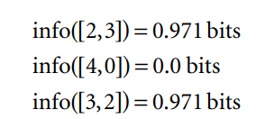
For outlook We can calculate the average information value of these, taking into account the number of instances that go down each branch—five down the first and third and four down the second:

This average represents the amount of information that we expect would be necessary to specify the class of a new instance, given the tree structure in Figure 4.2(a) Before we created any of the nascent tree structures in Figure 4.2, the training examples at the root comprised line yes and five no nodes, corresponding to an information value of

Thus the tree in Figure is responsible for an information gain of

The way forward is clear. We calculate the information gain for each attribute and choose the one that gains the most information to split on. In the situation of Figure 4.2,

Calculating information
Before examining the detailed formula for calculating the amount of information required to specify the class of an example given that it reaches a tree node with a certain number of yes’s and no’s, consider first the kind of properties we would expect this quantity to have:

1. When the number of either yes’s or no’s is zero, the information is zero.
2. When the number of yes’s and no’s is equal, the information reaches a maximum
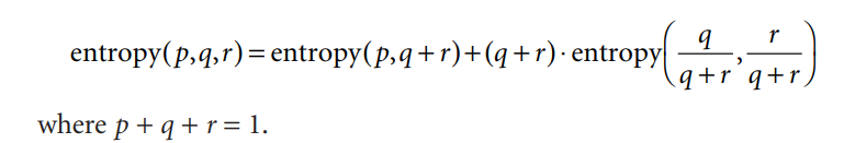
3. The information must obey the multistage property illustrated previously.
Remarkably, it turns out that there is only one function that satisfies all these properties, and it is known as the information value or entropy:

The arguments p1, p2, . . . of the entropy formula are expressed as fractions that add up to one, so that, for example, Info([2,3,4]) = entropy(2/3,3/9,4/9) Thus the multistage decision property can be written in general as
Because of the way the log function works, you can calculate the information measure without having to work out the individual fractions:

The method that has been described using the information gain criterion is essentially the same as one known as ID3. (https://en.wikipedia.org/wiki/ID3_algorithm)
A series of improvements to ID3 culminated in a practical and influential system for decision tree induction called C4.5 (https://en.wikipedia.org/wiki/C4.5_algorithm). These improvements include methods for dealing with numeric attributes, missing values, noisy data, and generating rules from trees.
Bibliography
Ian H. Witten, Eibe Frank. (1999). Data mining practical machine learning tools and techniques. Elsevier
